pyPOCQuant user manual
Introduction
The tool pyPOCQuant aims to automatically detect and quantify signal bands from lateral flow assays (LFA) or Point of Care tests (POC or POCT) from an image. It can batch analyze large amounts of images in parallel.
An analysis pipeline can be run either from the command line (good for automating large numbers of analysis) or from a desktop application.
![]()
Command line workflow
Split images by POCT manufacturer if needed
Copy all the images of the same kind into one folder
Prepare a settings (configuration) file
Run the pipeline
Split images by POCT manufacturer
This only applies if you collected many images using POCTs from different vendors and stored all the images in one common folder! Analysis settings would need to be slightly adapted for different POCTs shapes and sizes.
If you have many images in an unorganized way we provide a helper script to sort them by manufacturer into subfolders.
This can also be run from the UI, see below.
$ python ./split_images_by_strip_type_parallel.py -f /PATH/TO/INPUT/FOLDER -o /PATH/TO/OUTPUT/FOLDER -w ${NUM_WORKERS}
/PATH/TO/INPUT/FOLDER: path to the folder that contains all images for a given camera.PATH/TO/OUTPUT/FOLDER: path where all images will be organized into subfolders; one per each strip manufactured. Strip images that cannot be recognized (or do not contain any strip) will be moved to anUNDEFINEDsubfolder.Currently recognized manufacturers:
AUGURIXBIOZAKCTKBIOTECHDRALBERMEXACARELUMIRATEKNTBIOSUREBIOTECHTAMIRNA
Please notice: the list of known manufacturers is defined in pyPOCQuant.consts.KnownManufacturers.
NUM_WORKERS: number of parallel processes; e.g.8.
Settings file preparation
You can prepare a default parameter file from the command line as follows:
$ python ./pypocquant/pyPOCQuant_FH.py -c /PATH/TO/INPUT/settings_file.conf
Open the file in a text editor and edit it.
qc=True
verbose=True
sensor_band_names=('igm', 'igg', 'ctl')
peak_expected_relative_location=(0.25, 0.53, 0.79)
sensor_center=(178, 667)
sensor_size=(61, 249)
sensor_border=(7, 7)
perform_sensor_search=True
qr_code_border=40
subtract_background=True
sensor_search_area=(71, 259)
sensor_thresh_factor=2.0
raw_auto_stretch=False
raw_auto_wb=False
strip_try_correct_orientation=False
strip_try_correct_orientation_rects=(0.52, 0.15, 0.09)
strip_text_to_search='COVID'
strip_text_on_right=True
force_fid_search=True
Some of the parameter names contain the term
strip: this is used to indicate the POCT. The prefixsensorindicates the measurement region within thestrip.
See Explanations for detailed description of the parameters.
Please notice that some parameters are considered “Advanced”; in the user interface the parameters are separated into “Runtime parameters”, “Basic parameters”, and “Advanced parameters”.
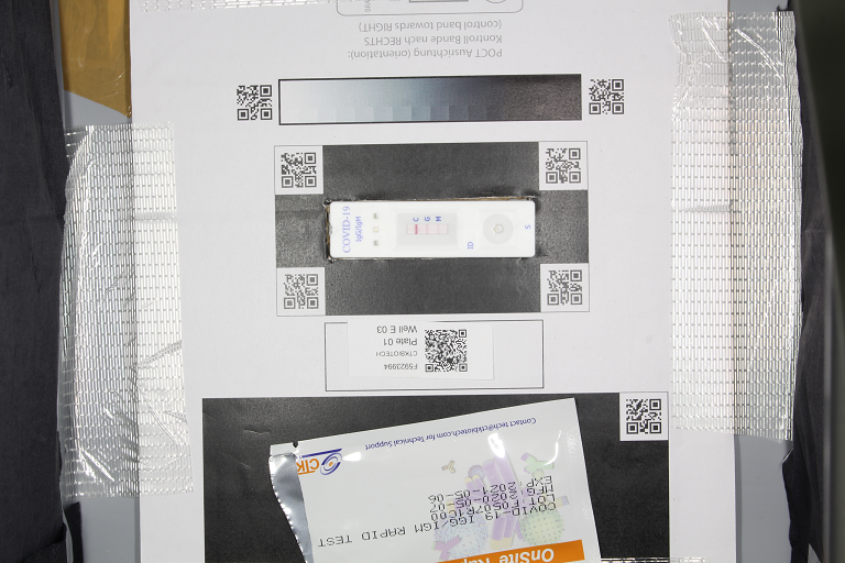
How to determine the parameters manually
Open the settings file and adjust the parameters to fit your images.
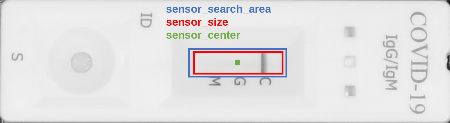
Important parameters are the sensor_size, sensor_center, and sensor_search_area (the latter being an advanced parameter).
The user interface allows to easily define those parameters by drawing onto the extracted POCT image.
Sensor parameters are relative to the POCT image.
In the following we show how to obtain position and extent of the sensor areas in Fiji or ImageJ. Later we will see how to do the same in the pyPOCQuant user interface.
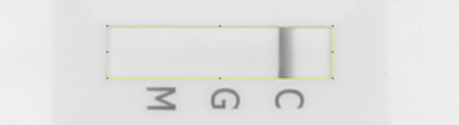
When drawing a rectangular region of interest, the size is displayed in Fiji’s toolbar; e.g.
x=539, y=145, **w=230, h=62**.When hovering over the central pixels in the top or left sides of the selection, the
x, andycoordinates of the center, respectively, are show in Fiji’s toolbar; e.g.x=*601*, y=144, value=214(and equivalently fory).
Run the pipeline
Run the analysis per manufacturer manually
$ python pyPOCQuant_FH.py -f /PATH/TO/INPUT/FOLDER/MANUFACTURER -o /PATH/TO/RESULTS/FOLDER -s /PATH/TO/CONFIG/FILE -w ${NUM_WORKERS}
/PATH/TO/INPUT/FOLDER/MANUFACTURER: path to the folder that contains all images for a given camera and manufacturer./PATH/TO/RESULTS/FOLDER: path where the results (and the quality control images) for a given camera and manufacturer will be saved. The results are saved in aquantification_data.csvtext file./PATH/TO/CONFIG/FILE: path to the configuration file to be used for this analysis. Please see below. Notice that a configuration file will be needed per manufacturer and (possibly) camera combination.NUM_WORKERS: number of parallel processes; e.g.8.
GUI workflow
Split images by POCT manufacturer if needed
Copy all the images of the same kind into one folder
Select the folder containing the images to be processed
Set all analysis parameters
Run the pipeline
Split images by POCT manufacturer
This only applies if you collected many images using POCTs from different vendors and stored all the images in one common folder! Analysis settings would need to be slightly adapted for different POCTs shapes and sizes.
To do so go to File –> Split images by type to open the dialog to split the images.
How to determine the parameters automatically using the GUI
A settings file must not necessarily be created in advance. The Parameter Tree can be edited directly. Optionally, settings can be loaded or saved from the UI.
How to estimate sensor parameters graphically in the UI:
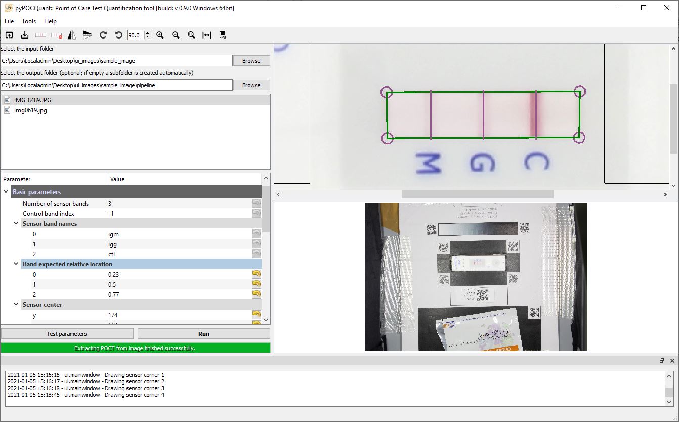
Select the input folderand click on one of the listed images to display it. The POCT region will be automatically extracted and shown in the view at the top. Please mind that this can take a few seconds. The lower view shows the whole image.Hit the
Draw sensor outlineicon (red arrow) in the toolbar. This will allow you to interactively define thesensor areaand thepeak_expected_relative_locationparameters.
Drawing sensor by clicking into the corners |
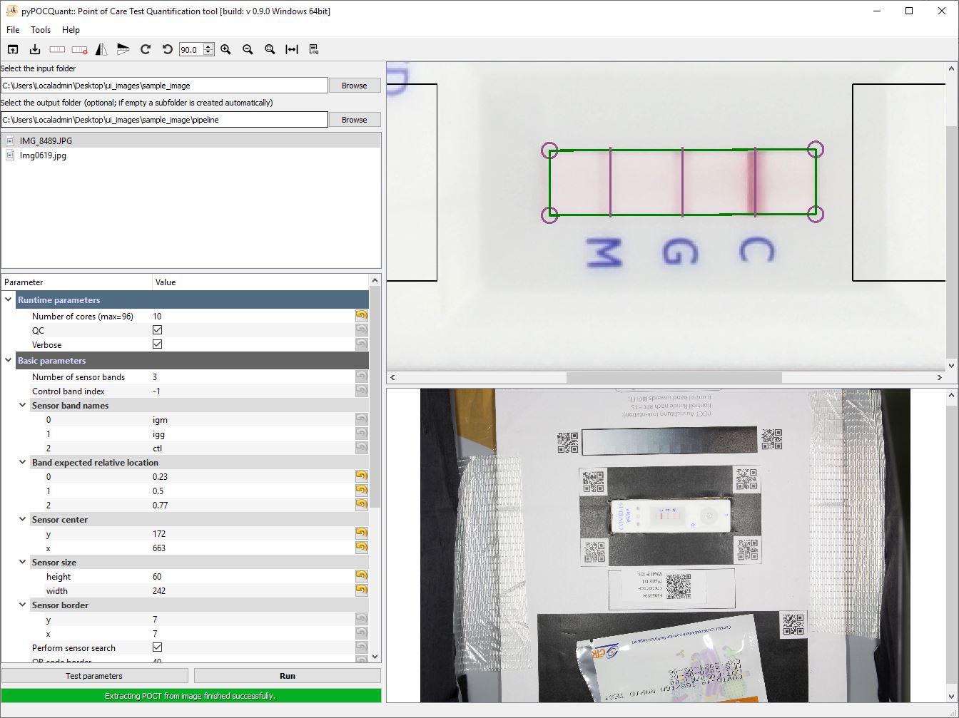
Drawing finished with aligned bars |
|---|---|
|
|
Draw the four corners of the sensor and place the vertical bars on the bands. This will cause all relevant parameters to be populated in the Parameter Tree. Please notice that, by default, the
sensor_search_areais set to be 10 pixels wider and taller than thesensor_size. This can be changed in the advanced parameters (but beware to keep it only slightly larger than thesensor_size: it is meant only for small refinements).
You can test current parameters on one image by clicking the
Test parametersbutton under the Parameter Tree.Optionally, you can save the settings file (Ctrl+S,
File->Save settings file)
Run the analysis per manufacturer automatically using the GUI
Once the previous steps are done and all parameters are correctly set, you can hit the Run button to start the analysis.
Note: a step by step guide can be found under **Quick start* (Help -> Quick start)*
Settings
The following settings must be specified. These are default values and need to be adopted for a series of the same kind of images. Please note: in the following, strip is used to indicate the POCT, and sensor to indicate the measurement region within the strip.
qc=True
verbose=True
sensor_band_names=('igm', 'igg', 'ctl')
peak_expected_relative_location=(0.25, 0.53, 0.79)
sensor_center=(178, 667)
sensor_size=(61, 249)
sensor_border=(7, 7)
perform_sensor_search=True
qr_code_border=40
subtract_background=True
sensor_search_area=(71, 259)
sensor_thresh_factor=2.0
raw_auto_stretch=False
raw_auto_wb=False
strip_try_correct_orientation=False
strip_try_correct_orientation_rects=(0.52, 0.15, 0.09)
strip_text_to_search='COVID'
strip_text_on_right=True
force_fid_search=True
Explanations
Runtime parameters
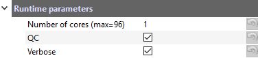
max_workers
The analysis can work in parallel. Specify the maximum number of images that are run in parallel. The maximum allowed value is the number of cores in your machine.
qc
Toggle creation of quality control images.
Possible values:
TrueorFalseRecommended:
Truewhen testing parameters.
verbose
Toggle extensive information logging.
Possible values:
TrueorFalseRecommended:
Truewhen testing parameters.
Basic parameters
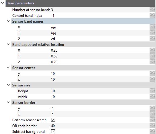
number_of_sensor_bands
It defines the number of test lines (TLs) to be expected in the POCT, including the control line. This parameter is used by the user interface to dynamically adapt the tree for related settings (see
sensor_band_namesandpeak_expected_relative_locationbelow), and is not part of the settings file, since it can be easily derived fro those parameters.Possible values:
2to100
control_band_index
Index of the control line.
Possible values:
0,1,...,number_of_sensor_bands - 1; or-1(last index).Default:
-1(in Python parlance,-1means last index, or, the first index from the right).
sensor_band_names
Custom name for the test lines (by default 3, needs to match the number of defined TLs
number_of_sensor_bands)t2,t1andctl(e.g.,IgM,IgGandCtl).
peak_expected_relative_location
Expected relative peak positions as a function of the width of the sensor (= 1.0). These values can easily be set interactively using the UI.
sensor_center
Coordinates in pixels of the center of the sensor with respect to the strip image:
(y, x).
sensor_size
Area in pixels of the sensor to be extracted:
(height, width).
sensor_border
Lateral and vertical sensor border in pixels to be ignored in the analysis to avoid border effects:
(lateral, vertical).
perform_sensor_search
If
True, the (inverted) sensor is searched withinsensor_search_areaaround the expectedsensor_center; ifFalse, the sensor of sizesensor_sizeis simply extracted from the strip image centered at the relative strip positionsensor_center.Possible values:
TrueorFalseRecommended:
True
qr_code_border
Lateral and vertical extension of the (white) border around each QR code.
subtract_background
If
True, estimate and subtract the background of the sensor intensity profile (bands).Possible values:
TrueorFalseRecommended:
True
Advanced parameters
These parameters will most likely work with the default values above.
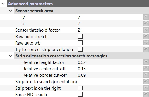
sensor_search_area
Search area in pixels around the sensor:
(height, width).Used only if
skip_sensor_searchisFalse.Try to keep it just a bit larger than the sensor size: in particular, try to avoid picking up features (e.g. text) in close proximity of the sensor.
sensor_thresh_factor
Set the number of (robust) standard deviations away from the median band background for a peak (band) to be considered valid.
Recommended:
2, maybe3.
raw_auto_stretch
Whether to automatically correct the white balance of RAW images on load. This does not affect JPEG images!
Possible values:
TrueorFalseRecommended:
False
raw_auto_wb
Whether to automatically stretch image intensities of RAW images on load. This does not affect JPEG images!
Possible values:
TrueorFalseRecommended:
False
strip_try_correct_orientation
Whether to automatically try to rotate a POCT that was mistakenly placed on the template facing the wrong direction (and where the control band is on the left instead of on the right). The pipetting inlet will be searched in the POCT; the inlet is assumed to be found on the side opposite to the control band, and always on the left. If found on the right, the image will be rotated.
Possible values:
TrueorFalseDefault:
FalseIf set to
True, make sure to properly set thestrip_try_correct_orientation_rectsparameters below!
strip_try_correct_orientation_rects
Parameters for defining two rectangles left and right from the sensor center to be used to detect the pipetting inlet. The first parameter,
Relative height factor, defines the relative height of the rectangles with respect to the strip. The second parameter,Relative center cut-off, defines the relative offset from the sensor center and therefore the width of the rectangle. Finally, the third parameter,Relative border cut-off, defines the relative offset from the strip’s left and right borders and hence the width of the search rectangle.Possible values:
(0:1, 0:1, 0:1)Default:
(0.52, 0.15, 0.09)
strip_text_to_search
Whether to use a specific text printed on the POCT to automatically try to rotate a POCT that was mistakenly placed on the template facing the wrong direction (and where the control band is on the left instead of on the right). Set to
""to skip search and correction. If the strip has some text printed on either side of the sensor, it can be searched to guess the orientation. See alsostrip_text_on_right.
strip_text_on_right
Assuming the strip is oriented horizontally, whether the
strip_text_to_searchtext is expected to be on the right. Ifstrip_text_on_rightisTrueand the text is found on the left hand-side of the strip, the strip will be rotated 180 degrees.Ignored if
strip_text_to_searchis"".
force_fid_search
If force fid search is activated, try hard (and slow!) to find an FID on a barcode or QR code label on the image identifying the sample.
Possible values:
TrueorFalseRecommended:
False
Results
The analysis pipeline delivers a .csv that contains a relatively large table of results. The extracted features are explained in the following.
Result table
Structure and description of the result table:
fid: patient FID in the form F5921788
fid_num: just the numeric part of the FID (i.e., 5921788)
filename: name of the analyzed image
extension: extension (either *.JPG or *.ARW, *.CR2, *.NEF)
basename: filename without extension
iso_date: date of image acquisition in the form YYYY-MM-DD (e.g. 2020-04-14)
iso_time: time of image acquisition in the form HH-MM-SS (24-h format)
exp_time: camera exposure time
f_number: aperture F number
focal_length_35_mm: 35mm equivalent focal length
iso_speed: camera ISO value
manufacturer: POCT manufacturer
plate: plate number
well: well (e.g. A 01)
ctl: 1 if the control band could be extracted, 0 otherwise.
t2: 1 if the t2 band (e.g. IgM) could be extracted, 0 otherwise.
t1: 1 if the t1 band (e.g. IgG) could be extracted, 0 otherwise.
ctl_abs: absolute signal strength of the control band,
t2_abs: absolute signal strength of the t2 band,
t1_abs: absolute signal strength of the t1 band.
ctl_ratio: relative signal strength of the control band (always 1.0 if detected)
t2_ratio: relative signal strength of the t2 band with respect to the control band
t1_ratio: relative signal strength of the t1 band with respect to the control band
issue: if issue is 0, the image could be analyzed successfully, if issue > 0 it could not. See the list of issues below
user: custom field
Note: expect small residual variations in the absolute signal strengths (
ctl_abs,t2_abs, andt1_abs) across images in a batch due to inhomogeneities in acquisition.Note 2:
ctl,t1, andt2in the column names will be replaced by the names defines insensor_band_names. For examples,t1_ratiomay becomeigg_ratio.Note 3: The number of test lines (TL) changes according to the parameter
number_of_sensor_bands. By default, 3 TLs are defined including thectlline. Changing the number of TLs also changes the number of columns in the results table.
Analysis issues
Each analyzed image is assigned an integer issue:
0: no issue, the analysis could be performed successfully
1: barcode extraction failed
2: FID extraction failed
3: strip box extraction failed
4: strip extraction failed
5: poor strip alignment
6: sensor extraction failed
7: peak/band quantification failed
8: control band missing
Quality control images
Types and examples’ of quality control images:
Raw image shown as comparison:
IMAGE_FILE_NAME_aligned_boxAligned raw image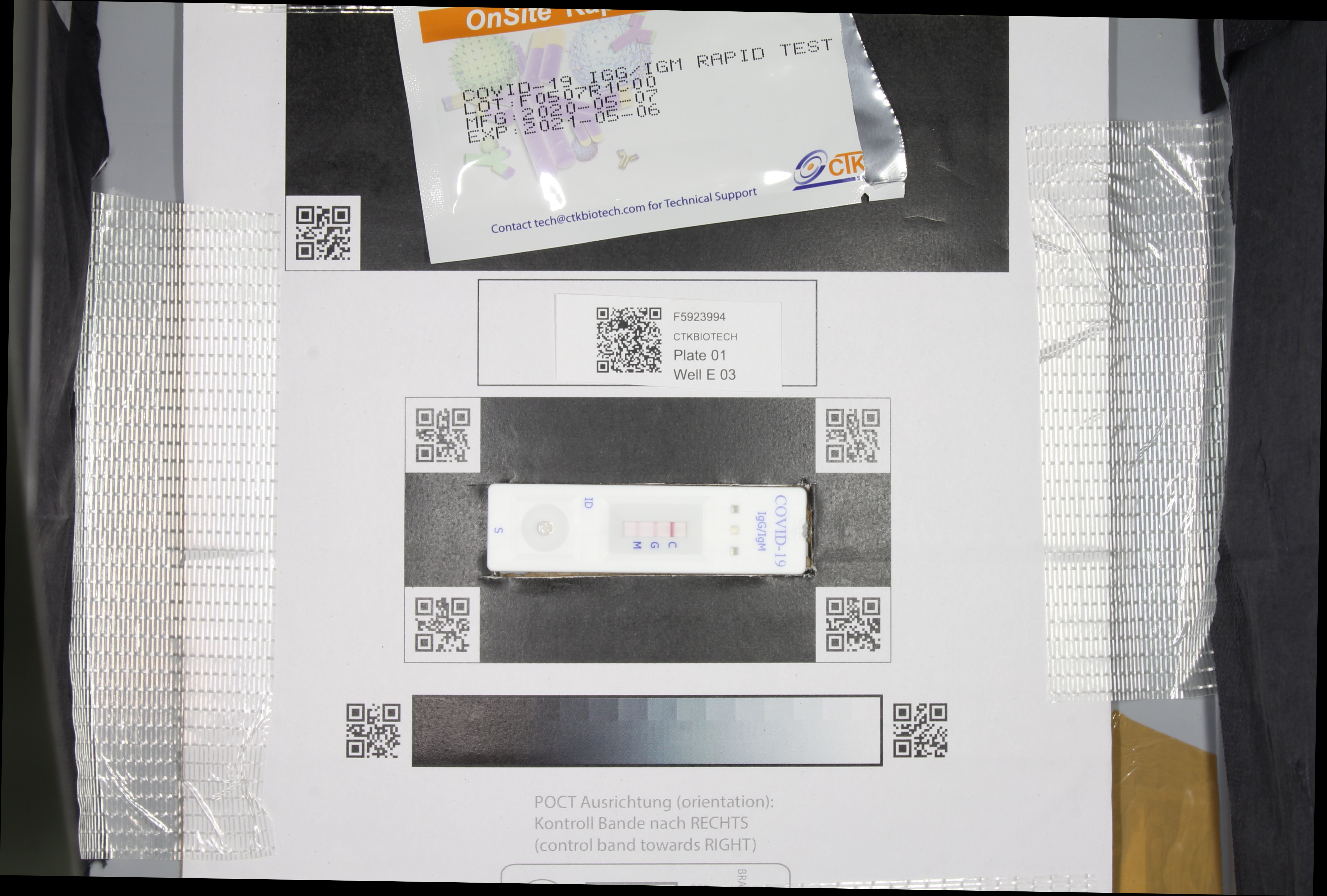
IMAGE_FILE_NAME_box: QR code box around the POCT oriented such that the control band is always on the right side.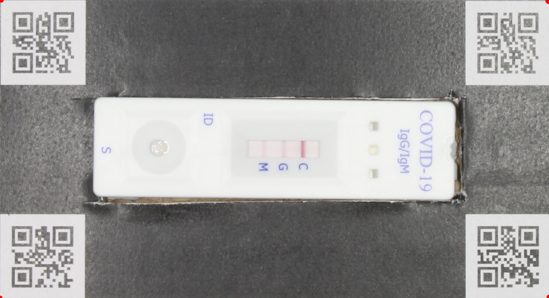
IMAGE_FILE_NAME_rotated: Raw image rotated such that the POCT is at the parallel to the bottom side of the image.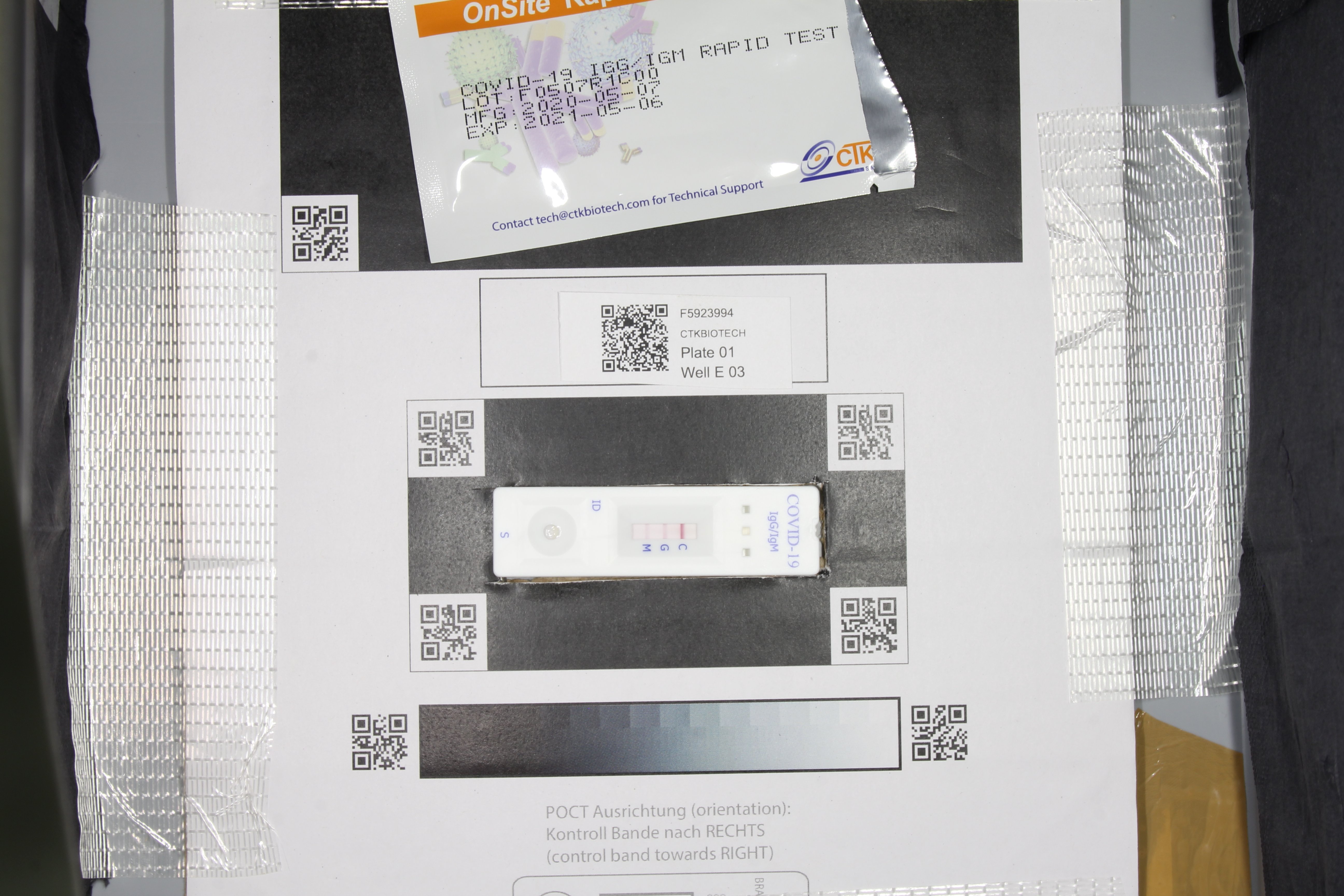
IMAGE_FILE_NAME_strip_gray_aligned: Aligned POCT cropped around its outline such that it is parallel to the bottom side.
IMAGE_FILE_NAME_strip_gray_aligned_after_ocrAligned POCT cropped around its outline such that it is parallel to the bottom side after OCR filtering such that the pipetting part is always left (for the cases where the POCT was not placed in the correct orientation in the template.)
IMAGE_FILE_NAME_strip_gray_hough_analysisAligned POCT cropped around its outline such that it is parallel to the bottom side detecting the pipetting spot to identify wrongly oriented POCT in the strip box.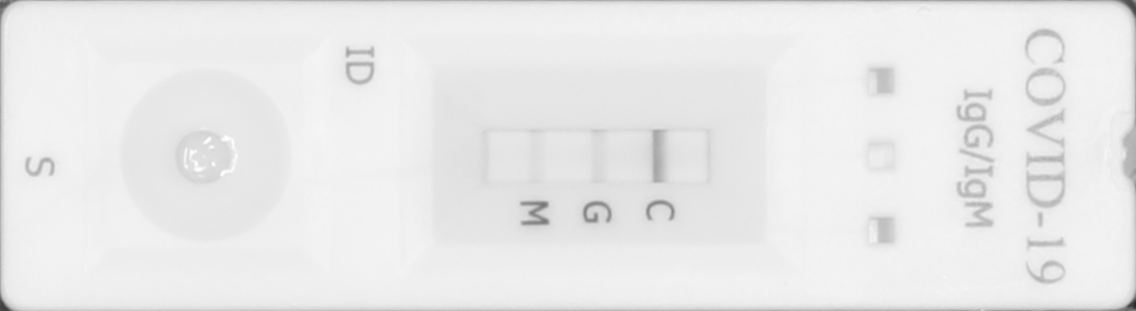
IMAGE_FILE_NAME_strip_gray_hough_analysis_candidatesHough analysis candidate results. The rectangles indicate the search areas while as the circles indicate potential hits for the pipetting spot. Red rectangle and magenta circles identifies the side where the pipetting spot was detected. Note it is assumed that the control band is always opposite of the pipetting area.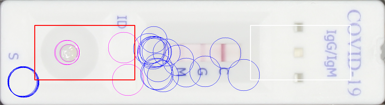
IMAGE_FILE_NAME_sensor: Aligned sensor crop showing the bands.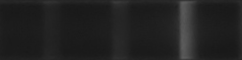
IMAGE_FILE_NAME_peak_overlays: Sensor crop with colored rectangle overlay(s) indicating the area(s) where the signal for each detected band is quantified. Notice that the rectangle extends to cover the whole area under the curve, from background level through peak and back to background level.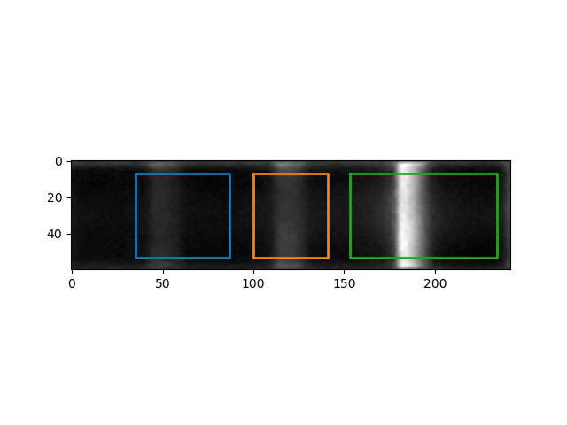
IMAGE_FILE_NAME_peak_background_estimation: Control figure displaying the performance of the background estimation fit. Black dashed line is a an estimation of the background level obtained by robust linear fit of the band profile. From the estimate background trend a constant value is subtracted (resulting red solid line). This is to make sure that the signal is flat after correction, but no values are clipped.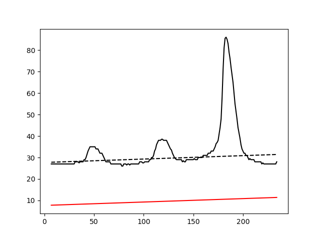
IMAGE_FILE_NAME_peak_analysis: Control figure displaying the performance of the peak analysis. Red circle indicates the max peak height. The green dashed line is an estimate of the local background that is used to test all candidate local maxima against a threshold defined by the red dashed line. This line is calculated as the (median of the background values) +f* (median deviation of the background values). The factorfis a user parameter and defaults to 2. The solid blue, orange and green line under the curves indicate the local span of each of the bands and indicate which part of the signal is integrated.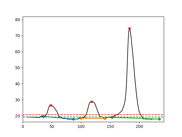
Log file
The log file contains more detailed information for each processed image identified by its file name, such as IMG_8489.JPG.
It informs about barcode extraction and its rotation, QR code box rotation, FID extraction, actual sensor coordinates and the identified bands.
Example log:
File = IMG_8489.JPG
Processing IMG_8489.JPG
Best percentiles for barcode extraction: (0, 100); best scaling factor = 0.25; score = 6/6
File IMG_8489.JPG: best percentiles for barcode extraction after rotation: (0, 100); best scaling factor = 0.25; score = 6/6
File IMG_8489.JPG: Strip box image rotated by angle -0.9172186022623166 degrees using QR code locations.
File IMG_8489.JPG: FID = 'F5923994'
File IMG_8489.JPG: sensor coordinates = [140, 207, 523, 780], score = 1.0
Peak 69 has lower bound 48 (d = 21) with relative intensity 0.06 and upper bound 93 (d = 24) with relative intensity 0.00. Band width is 46. Band skewness is 1.14
Peak 138 has lower bound 104 (d = 34) with relative intensity 0.00 and upper bound 162 (d = 24) with relative intensity 0.10. Band width is 59. Band skewness is 0.71
Peak 203 has lower bound 170 (d = 33) with relative intensity 0.04 and upper bound 248 (d = 45) with relative intensity 0.00. Band width is 79. Band skewness is 1.36
File IMG_8489.JPG: the bands were 'normal'.
✓ File IMG_8489.JPG: successfully processed and added to results table.
Settings file
A settings file is created in the -o /PATH/TO/RESULTS/FOLDER with the actually used parameters for the analysis. It can be used to reproduce the obtained results.
See settings file section for detailed description.
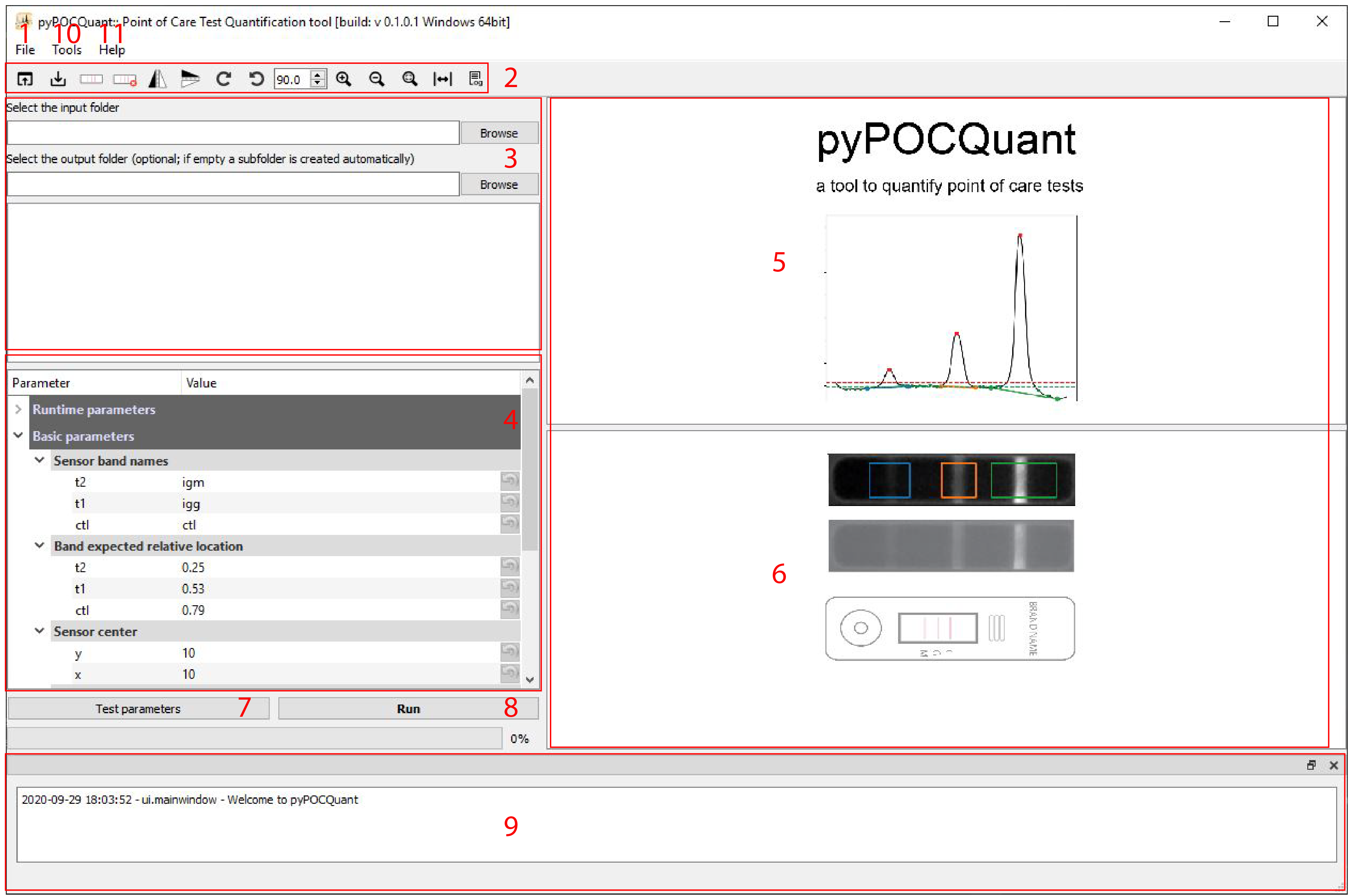
Graphical user interface
The GUI offers several actions via the menu, the toolbar and buttons.
File menu: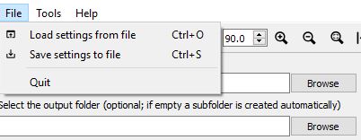
File: Lets you load (File–>Load settings file) and save (File–>Save settings file) a settings fileHelp: Get quick instructions and open this manual
Toolbar:
Load settings from file: Load settings from file into the Parameter Tree.Save settings to file: Save current settings to file.Draw sensor outline: Activates drawing a polygon by clicking into the corners of the sensor on the images.Delete sensor: Deletes currently drawn sensor.Mirror image vertically: Mirrors the displayed image vertically.Mirror image horizontally: Mirrors the displayed image horizontally.Rotate clockwise: Rotates the displayed image clock wise.Rotate counter clockwise: Rotates the displayed image counter clock wise.Set rotation angle in degrees: Specifies the rotation angle.Zoom in: Zooms in the displayed image.Zoom out: Zooms out the displayed image .Reset zoom: Resets the zoom level.Measure distance: Lets you draw a line on the image to measure distances. It will update theqr_border_distanceparameter.Show / hide console: shows or hides the console at the bottom of the UI.
Select input folder: Allows to specify the input folder.Select output folder: (Optional) Lets you select a output folder. If left empty a output subfolder is automatically generated in the input folder.Image list: Lists all available images in the input folder. Click onto the filename to display one in 5.Parameter Tree: Adjust parameters manually if needed.POCT area: Shows the extracted POCT and allows for drawing the sensor.Display area: Shows the currently selected image.Test parameters: Runs the pipeline on the selected image with current settings. The test folder will be opened automatically to inspect the control files.Run: Runs the pipeline with the current settings**.Log: Informs the user about performed actions.Tools menu: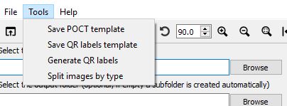
Save POCT template: Lets you save and print the POCT template to be used for the image acquisition.Save QR labels templateLets you save an Excel template to be used to generate QR code labels for all your samples from a list.Generate QR labels: Lets you generate QR labels for your samples using the excel template or a csv file with a list of the names in the correct format:
SAMPEID-MANUFACTURER-PLATE-WELL-USERDATA. You can use theUSERDATAfield for very short annotations; please make sure not to use dashes (-) in this field, but replace them with underscores (_). You can define the page size, label size, position and number per page to match the format for any printable label paper as, for instance, from AVERY.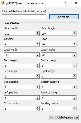
Split images by type: helps organizing mixtures of images from different POCT manufacturers stored in one and the same folder. The tool will analyze each of the images and attempt to extract the manufacturer information from the QR code (if present) or by searching for the name on the POCT itself (OCR). If the manufacturer can be resolved, the image is moved into a sub-folder with the name of the manufacturer, otherwise it will be moved into a subfolder called UNDEFINED. As long as the QR code structure is satisfied (which is guaranteed if using theGenerate QR labelstool explained above), even previously unknown manufacturers can be recognized. Should the QR code detection fail, a fall-back OCR detection can use a comma-separated list of expected manufacturer names to potentially identify unknown manufacturers. Theinput folderdefines the folder containing all the images to process, andoutput folderthe location where the split images should be moved. Thenumber of coresdefines the number of images that will be processed in parallel.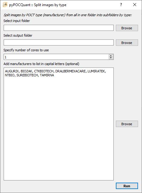
Help menu: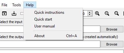
Quick instructions: Shows the quick instructions dialog.Quick start: Opens the quick start document describing how to set up the image acquisition setup, perform the acquisition and some potential problems and their solutions one might encounter.User manual: Opens this document.About: About the software and its dependencies.